K-means Clustering Python Example

Machine Learning Algorithms: K-Means Example In Sklearn Python

K-Means Clustering is an unsupervised machine learning algorithm. In contrast to traditional supervised machine learning algorithms, K-Means attempts to classify data without having first been trained with labeled data. Once the algorithm has been run and the groups are defined, any new data can be easily assigned to the most relevant group.

The real world applications of K-Means include:

• customer profiling
• market segmentation
• computer vision
• search engines
• astronomy

How it works

1. Select K (i.e. 2) random points as cluster centers called centroids

2. Assign each data point to the closest cluster by calculating its distance with respect to each centroid

3. Determine the new cluster center by computing the average of the assigned points

4. Repeat steps 2 and 3 until none of the cluster assignments change

Choosing the right number of clusters

Often times the data you’ll be working with will have multiple dimensions making it difficult to visual. As a consequence, the optimum number of clusters is no longer obvious. Fortunately, we have a way of determining this mathematically.

We graph the relationship between the number of clusters and Within Cluster Sum of Squares (WCSS) then we select the number of clusters where the change in WCSS begins to level off (elbow method).

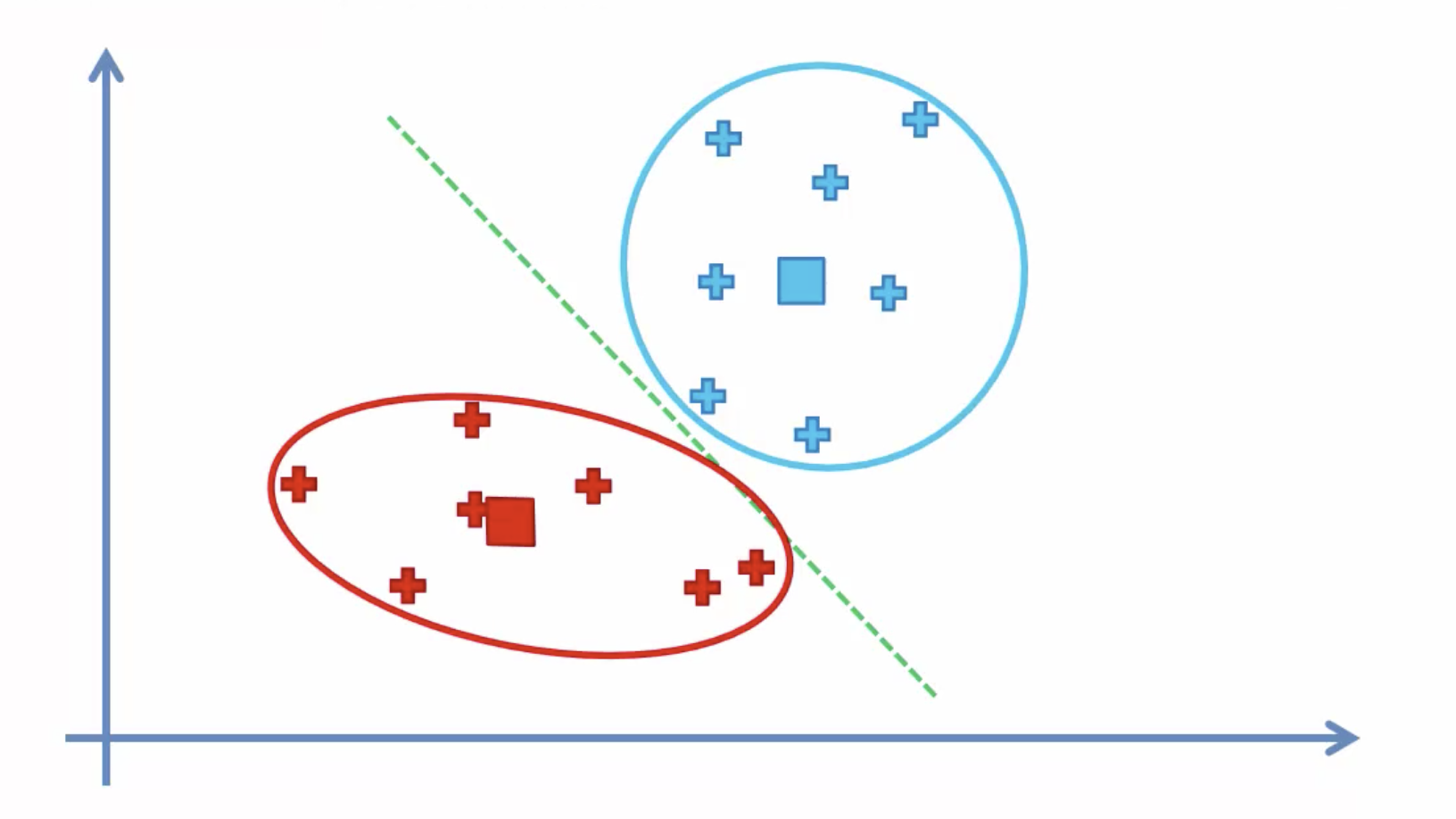
WCSS is defined as the sum of the squared distance between each member of the cluster and its centroid.

For example, the computed WCSS for figure 1 would be greater than the WCSS calculated for figure 2.

Code

Let’s take a look at how we could go about classifying data using the K-Means algorithm with python. As always, we need to start by importing the required libraries.

import numpy as np  
import pandas as pd  
from matplotlib import pyplot as plt  
from sklearn.datasets.samples_generator import make_blobs  
from sklearn.cluster import KMeans

In this tutorial, we’ll generate our own data using the make_blobs function from the sklearn.datasets module. The centers parameter specifies the number of clusters.

X, y = make_blobs(n_samples=300, centers=4, cluster_std=0.60, random_state=0)

plt.scatter(X[:,0], X[:,1])

Even though we already know the optimal number of clusters, I figured we could still benefit from determining it using the elbow method. To get the values used in the graph, we train multiple models using a different number of clusters and storing the value of the intertia_ property (WCSS) every time.

wcss = []

for i in range(1, 11):  
    kmeans = KMeans(n_clusters=i, init='k-means++', max_iter=300, n_init=10, random_state=0)  
    kmeans.fit(X)  
    wcss.append(kmeans.inertia_)  
plt.plot(range(1, 11), wcss)  
plt.title('Elbow Method')  
plt.xlabel('Number of clusters')  
plt.ylabel('WCSS')  
plt.show()

Next, we’ll categorize the data using the optimum number of clusters (4) we determined in the last step. k-means++ ensures that you get don’t fall into the random initialization trap.

kmeans = KMeans(n_clusters=4, init='k-means++', max_iter=300, n_init=10, random_state=0)  
pred_y = kmeans.fit_predict(X)

plt.scatter(X[:,0], X[:,1])  
plt.scatter(kmeans.cluster_centers_[:, 0], kmeans.cluster_centers_[:, 1], s=300, c='red')  
plt.show()